Uvisensor package

client.py
This module contains the Client class, which inherits from socket.socket
- socket.socket class source code can be found in the following link: https://hg.python.org/cpython/file/2.7/Lib/socket.py
- Previous class is a child of the _socket.socket class. Its source code can be found in the following link: https://github.com/biosbits/bits/blob/master/python/_socket.py
-
class
uvisensor.client.Client(buffer_size=2048, timeout=2.0)¶ Child class of socket.socket which includes register operations.
It is intended to work with registers of an external FPGA. The register identifiers must correspond with the ones of the HDL circuit implemented in the FPGA.
Used methods from parent class:
- connect((host, port)): connects to specified remote address
- close(): close the socket opened with the client
- send(data): send data to the client
- recv(buflen): read the specified number of bytes
- settimeout(timeout): time to wait for the client to respond
Parameters: - buffer_size (int) – number of bytes of the incoming data.
- timeout (int or float) – value, in seconds, of the time that will be waited for reading incoming data. This will set the object to timeout mode (By default, it is set to blocking mode).
The class has 2 dictionaries, _REGISTERS and _COMMANDS, that contain all the valid commands that can be sent to the FPGA and the declared registers inside it. When interacting with the FPGA, can only be accessed the commands and registers in these dictionaries.
Registers
- RED/GREEN/BLUE_THRESHOLD: The pixel intensity thresholds for each of the 3 colors are stored in these registers, in the form of (low_threshold, high_threshold).
- IMAGE_SHAPE:
- ...
-
close_connection()¶ Send ‘CLOSE_CONNECTION’ command to FPGA and close TCP/IP socket.
-
open_connection(ip, port)¶ Create a TCP/IP socket connection.
After connecting, the input buffer is read in order to remove its contents, as a ‘Welcome message’ is automatically generated.
Parameters: - ip (str) – IP address of the device.
- port (int) – socket port.
-
read_data(size)¶ Perform the input buffer read operation several times.
Parameters: size (int) – indicates number of bytes to be read. Returns: A data concatenation of all packages read from the input buffer.
-
read_register(regkey)¶ Read the value of a register and return it formatted.
Parameters: regkey (str) – register identifier Returns: the content of the register Return type: int or list
-
write_command(command, clean_buffer=False)¶ Send a command to the TCP/IP client.
Parameters: - command (str) – FPGA command to be executed.
- clean_buffer (bool) – if True, a clean-up reading of the input buffer is done after writing.
Returns: message returned from the FPGA after writing the command. If clean_buffer is False or there was no message, ‘EMPTY_BUFFER’ is returned.
-
write_register(regkey, value)¶ Write a value into a register and clean the input buffer.
Parameters: - regkey (str) – register identifier that will be written.
- value – data that will be written to the register. It will be converted to a string before sending.
Returns: message given back by the FPGA after writing the register
geometry.py
This module contain classes and methods with geometrical operations.
The operations are done in the 2-D space It works with 2-D shapes represented by arrays. Thus, the calculations are based on matrix operations and linear algebra.
-
class
uvisensor.geometry.Triangle(vertices, isglobal=False, cartesian=False)¶ Class for dealing with geometric operations referred to triangles.
An instance of the class represents an isosceles triangle in a 2-D space, with the 2 equal sides being bigger than the base one.
Parameters: - vertices (np.array(shape=3x2)) – vertices coordinates of the triangle object.
- isglobal (bool) – Flag that indicates if the coordinate system refers to the 4-quadrant system (global) or to a local quadrant system.
- cartesian (bool) – This flag indicates if the coordinates are referred to a cartesian system [x,y] instead of the images typical standard [row. column] = [y,x]
-
get_pose()¶ Return triangle’s angle and base midpoint, given its vertices.
The coordinates of 3 vertices defining the triangle are used, packed in a single 3x2 array. This method assumes that the triangle is isosceles and the 2 equal sides are bigger than the different one, called base.
The following attributes are updated:
- self.sides : array containing the lengths of the 3 sides.
- self.base_index : array index of the minor side. This is also the index of the vertex between the 2 mayor sides, as vertices indexes are the indexes of their opposite sides.
Returns: [X,Y] coordinate of the midpoint of the triangle’s base side and orientation angle of the triangle. It is the resulting angle between the horizontal axis and the segment that goes from the triangle’s midpoint to the frontal vertex. It is expressed in radians, in the range [-pi, pi]. Return type: float32, float32, float32
-
get_window(min_value, max_value, k=1.25)¶ Get the coordinates of a rectangle window around the triangle.
At first, the barycenter of the triangle is calculated. Then, the window is calculated as a square, being its sides’ length k times the triangle’s longest side length and being its center the triangle’s barycenter. The output is stored in the self.window variable
Parameters: - min_value (int or np.array[int,int]) – value or values of the minimum allowed coordinates.
- max_value (int or np.array[int,int]) – value or values of the maximum allowed coordinates.
- k (int or float) – relative size between the window and the triangle base. It should be bigger than 1. As bigger as it gets, the bigger the window will be.
Returns: array representing a square parallel to the horizontal coordinates axe. The first row contains the X and Y minimum values of the square, and the second row contains its X and Y maximum values.
Return type: 2x2 np.array
-
global2local(offsets, K=None, cartesian2image=True)¶ Convert Triangle coordinates to the local coordinates system.
Only absolute coordinates shall be transformed. Lengths and angles are invariant to the coordinate origin.
Parameters: - offsets (list[int, int]) – column and row offsets between the local and the global systems.
- K (positive int or float) – Scale ratio to be applied to the points coordinates.
- cartesian2image (bool) – If True, a conversion from cartesian coordinates system to image system is performed. Thus, the output will be of the form of [row,column] instead of [x,y].
Raises: ValueError – if the scale ratio is negative.
-
homography(H)¶ Perform an homography operation to the Triangle vertices.
The homography is a geometrical transformation that obtains the projection of certain points from a plain to another. self.vertices variable is updated
Parameters: H (np.array(shape=3x3)) – Homography matrix. Returns: the new vertices coordinates values.
-
in_borders(limits, tolerance=150)¶ Evaluate if vertices are near a 4-sides polygon perimeter.
In the real world scenario, this method determines if the UGV, represented by the Triangle, is in the borders region of a given 2-D space, defined by an irregular 4-sides polygon.
Parameters: - limits (iterable of length 4) – Array containing the coordinates of the 4 points defining the borders of the polygon.
- tolerance (int or float) – Maximum allowed distance (mm) to the limits to be considered within the borders region.
Returns: flag set to True if the triangle is evaluated to be inside the given polygon
Return type: bool
-
inverse_homography(H)¶ Perform an inverse homography operation to the vertices.
Get
 from the equation
 .
.First of all, get
 using least
squares method. Then, extracts
using least
squares method. Then, extracts  from the
column matrix, with the hypothesis that
from the
column matrix, with the hypothesis that  .
.Parameters: H (np.array(shape=3x3)) – Homography matrix. Returns: the new vertices coordinates values.
-
local2global(offsets, K=None, image2cartesian=True)¶ Convert Triangle coordinates to the global coordinates system.
The function performs 2 transformations:
- Obtains the 4-quadrant coordinates. The input is a coordinate for a 1-quadrant system, and the output corresponds to the 4-quadrant system.
- Move y-axis origin. Initially, for a given image the origin is placed at its top. However, for the used system the origin is placed at the middle of the 4 quadrants.
If indicated, the coordinates system will be transformed to the cartesian one. This is recommended, as the image system does not make sense for a space with origin in the middle.
Only absolute coordinates shall be transformed. Lengths and angles are invariant to the coordinates origin.
Finally, a scale ratio K will be applied to the coordinates. The coordinates will be directly multiplied by the ratio.
Parameters: - offsets (list[int, int]) – column and row offsets between the local and the global systems.
- K (positive int or float) – Scale ratio to be applied to the points coordinates.
- image2cartesian (bool) – If True, a conversion from image coordinate system to cartesian system is performed. Thus, the output will be of the form of [x,y] instead of [row,column].
Raises: ValueError – if the scale ratio is negative.
-
class
uvisensor.geometry.Segment(point_a, point_b)¶ This class contains methods for dealing with 2D segments operations.
Parameters: - point_a (len-2 tuple or list) – X and Y coordinates of the initial points.
- point_b (len-2 tuple or list) – X and Y coordinates of the end points.
-
distance2point(point)¶ Return the distance of a point to the nearest segment’s point.
The calculus is based on the dot (scalar) product. The perpendicular projection of a first vector on a second one is the dot product the 2 vectors divided by the modulus of the second:

being
 the projection of A on B
If the projection is less than 0, it implies that the point is left to the first point (as cos(alpha) is negative), being this first point the nearest one to the target point.
Moreover, if the projection is greater than the modulus of the segment, it implies that the target point is is right to the end point, being this the nearest one.
Finally, the the distance to the segment is obtained and returned using the Pythagoras’ theorem.
Returns: The distance of the point to the segment
imgprocessing.py
This module contains the Image class, for image processing operations.
The operations implemented in the class methods are focused to the images obtained from the external FPGAs in the UviSpace project. Thus, once obtained a grey scale image, this module provide functions for getting the shapes (triangles) in the image, and then their vertices. Prior to segment the image, a binarization has to be applied, as it eases the segmentation process.
Important note
A point array is written by convention in the form [row, column]. In a cartesian system, the points are expressed as (x,y). Finally, in an image representation (viewer), the typical is to display points coordinates as (x’, y’). They equivalences are the following:
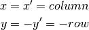
Thus, special care has to be taken when dealing with operations in different scopes e.g. trigonometric operations will be handled with the cartesian values, while image operations are normally performed with the array convention. Finally, when sending the array values to a viewer or to an external device, the image representation mentioned above is the typical used system.
-
class
uvisensor.imgprocessing.Image(image, contours=[])¶ Class with image processing methods oriented to UGV detection.
Parameters: - image (np.array) – original grey scale image.
- contours (list) – each element is an Mx2 array containing M points defining a closed contour.
-
binarize(thresholds)¶ Get a binarized image from a grey image given the thresholds.
The input image can only have one dimension. This method is intended to work with 3-component threshold values stored in a single 30-bit register:
- register[0 to 10] : red component thresholds
- register[10 to 20] : green component thresholds
- register[10 to 30] : blue component thresholds
The raw binary image contains a lot of noise. As it is very low around the triangles, masks around them are used to get rid of the noise in the rest of the image.
- :param [int or float, int or float] thresholds : minimum and
- maximum values between whom the image intensity values will be accepted as 1 (rescaled to 255). Values greater than the maximum and smaller than the minimum will be truncated to 0.
Return bin_image: Image of the same size as the input image with only 255 or 0 values (Equivalent to 1 and 0), according to the input threshold values. Return type: binary numpy.array(shape=MxN)
-
correct_distortion(kx=0.035, ky=0.035, only_contours=True)¶ Correct barrel distortion on contours or on the whole image.
The distortion is corrected using a 2nd polynomial equation for every pixel with coordinates
 . The resulting
corrected coordinates
. The resulting
corrected coordinates  are obtained with the
following equations:
are obtained with the
following equations:![X_u &=(X_d - C_x) * (1 + k_x * r^2) + C_x \
Y_u &= (Y_d - C_y) * (1 + k_y * r^2) + C_y \
r &= [(X_d - C_x)^2 + (Y_d - C_y)^2] / [(C_x^2 + C_y^2) * 2]](_images/math/4994570b3040808b7bf890686e1d4ebdc5e321c0.png)
Parameters: - kx (float) – X-Axe Distortion coefficient of the lens.
- ky (float) – Y-Axe Distortion coefficient of the lens.
- only_contours (bool) – Specify if the correction is to be applied to the whole image or only to the contours.
-
get_shapes(tolerance=8, get_contours=True)¶ Get the shapes’ vertices in the binarized image.
Update the self.triangles attribute.
The shape is obtained using the Marching Cubes Algorithm. Once obtained, the vertices are calculated using the Ramer-Douglas-Peucker Algorithm. Both are implemented on the skimage library, and there is more information on its docs.
if the kwarg get_contours if False, it is assumed that the contours are already known (stored in variable self.contours). If this is the case, the marching cubes algorithm is omitted.
Parameters: - tolerance (float) – minimum distance between an observed pixel and the previous vertices pixels required to add the first one to the vertices list.
- get_contours (bool) – specify if the Marching Cubes Algorithm is applied to the binarized image. Specifically set to False when the binarization algorithm is implemented in the external device (i.e. the FPGA).
Returns: vertices of the N shapes detected on the image. each element contains an Mx2 np.rray with the coordinates of the M vertices of the shape.
Return type: list
videosensor.py
This module contains the VideoSensor class and related functions.
The functions are calls to the VideoSensor class methods in order to capture images and then work with them using the imgprrocessing.Image class and its methods.
-
class
uvisensor.videosensor.VideoSensor(filename='', scale=2.0)¶ This class contains methods for dealing with FPGA-camera system.
Parameters: - filename (str) – Path to the configuration file of the camera. The path shall be passed relative to this script directory.
- scale (float) – scale ratio of the camera. relationship between the full resolution of the FPGA and the actual resolution that is being usedd. By, default, the FPGA has a 2:1 scale i.e. only half of the pixels are being used.
-
capture_frame(gray=True, tries=20, output_file='')¶ This method requests a frame to the FPGA.
Parameters: - gray (bool) – if true, a gray-scale image will be requested. If false, the requested image will be RGB.
- tries (int) – number of times that the system will try to obtain the requested image. After the last try, the system will exit.
- output_file (str) – URL name of the output file were the image will be stored. If left blank, the image won’t be saved.
Returns: image contained in an array with dimensions specified in the configuration file. If gray color is True, the dim value will be 1, and 3 for False (representing color images). dim equals to the number of components per pixel.
Return type: MxNxdim numpy.array
-
configure_tracker(tracker_id, min_x, min_y, width, height)¶ Send to FPGA rectangle parameters for defining a tracker.
Parameters: - tracker_id (int) – identifier of the detected object.
- min_x (int) – value of the X cartesian coordinate of the tracker window.
- min_y (int) – value of the Y cartesian coordinate of the tracker window.
- width (int) – value of the width (X axis) of the tracker window
- height (int) – value of the height (Y axis) of the tracker window.
NOTE: It is mandatory that the coordinates and dimensions passed to the FPGA are integers. Other types like float are not valid and the FPGA will not recognize them.
-
connect_client()¶ Read TCP/IP parameters in config file and connect to the device.
-
disconnect_client()¶ Close TCP/IP connection with the device.
If disconnect_client() function is not called, the socket won’t be able to be reopened.
-
get_homography_array()¶ Get an homography array from the configuration file.
-
get_limits_array()¶ Get the limits array from the configuration file.
-
get_offsets()¶ Get the offset of the sensor respect to the iSpace center.
The row offset of the camera images corresponds to the images height and the column offset corresponds to the images width.
Returns: row and column offsets i.e. [row_offset, col_offset] Return type: list[float, float]
-
get_register(register)¶ Read the content of the specified register.
Parameters: register (str) – key identifier of a valid register name of the FPGA. The full list of valid keys and their associated name can be found on the documentation of the client.Client class. Returns: the data stored in the indicated register.
-
load_configuration(write2fpga=True)¶ Load the config file and send the configuration to the FPGA.
- Read camera and sensor parameters in self.filename. They are then stored in the self._params variable.
- If write2fpga flag is True, write parameters in the FPGA registers by calling set_register() method. Finally, send ‘CONFIGURE_CAMERA’ command to FPGA.
-
read_conffile(filename)¶ Look for a configuration file on the given path and read it.
-
set_register(register, value)¶ Write a value into an FPGA register.
Parameters: - register (str) – key identifier of valid register name of the FPGA. The full list of valid keys and their associated name can be found on the documentation of the client.Client class.
- value (int or tuple/list) – the value that will be written to the register. It is mandatory to send it as string type. Thus, the value has to be converted. For tuples or lists, brackets or parenthesis are not allowed, so they have to be eliminated.
Returns: message obtained back from the FPGA after writing into the register.
Examples: - sent_value = ‘6’ —> OK
- sent_value = ‘(3.45, 2.21)’ —> No OK
- sent_value = ‘3.45, 2.21’ —> OK
kalmanfilter.py
Module with a class for implementing a Kalman filter.
The Kalman filter is a well-known algorithm for improving the localization of an object given measures of its position and a model of its behaviour.
The algorithm is defined by two main stages, i.e.: the state prediction, that estimates the state (position) of the object given the previous one and the value of the input variables; and the fusion with the measurements, that filters the values obtained by the sensors and the prediction calculated on the previous stage.
Relevant documentation:
-
class
uvisensor.kalmanfilter.Kalman(var_dim=3, input_dim=2)¶ Class for implementing a linear Kalman Filter.
It contains two methods for implementing the two stages of the Kalman filter (predict and update), that should be run alternating each one; and two methods for updating the noise matrices.
The noise distributions can be changed before the update stage, and the Kalman gain will vary accordingly.
-
predict(ext_input, delta_t)¶ Estimate the new position given the external input vector.
The matrix B, that maps input values to the corresponding state change, is directly proportional to the time step since the last iteration.
The function predicts the new position of the object, applying the input vector to the previous state. The function resolves the predicted position using 2 equations, one for the mean value and the other one for the covariance matrix:

Hypothesis: The angular speed between two iterations does not affect on the new position (x,y) of the object, as the time is considered small enough between iterations.
Parameters: - ext_input (np.array(shape = (input_dim x 1))) – values of the control variables.
- delta_t (float) – time step between the current iteration and the previous one.
Returns: The predicted state means, and the predicted covariance matrix.
-
set_measurement_noise(noise)¶ Set the measurement noise matrix to the given values
A bigger measurement noise will make the Kalman filter to diminish the weight of the state measurement given by the system sensors.
If the noise is uncorrelated, the input can be a tuple or list, and the output will be a diagonal matrix with the given values.
Note that the input dimensions must coincide with the dimensions of the system state variables.
Parameters: noise ('var_dim' length list or tuple; or a np.array(shape = (var_dim x var_dim))) – new values for the measurement noise. Returns: the new measurement error matrix.
-
set_prediction_noise(noise)¶ Set the prediction noise matrix to the given values
A bigger estimation or prediction noise will make the Kalman filter to diminish the weight of the state prediction on the final result.
If the noise is uncorrelated, the input can be a tuple or list, and the output will be a diagonal matrix with the given values.
Note that the input dimensions must coincide with the dimensions of the system state variables.
NOTE: A more more accurate model would calculate the process (prediction) noise depending on the magnitude of the input variables. According to the propagation of errors theory, the error of a multiplication is bigger when each of the products is bigger i.e. in this case, the predicted position error is bigger when the speeds are bigger (also when the time difference is bigger).
Parameters: noise ('var_dim' length list or tuple; or a np.array(shape = (var_dim x var_dim))) – new values for the process noise. Returns: the new process error matrix.
-
update(measurement)¶ Update the UGV position, merging the measurement and prediction
This is the second stage of the Kalman filter. Prior to applying it, the ‘predict’ stage has to be run, in order to obtain an estimated position and compare with the given measurement (‘z’).
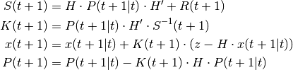
The final filtered position will be a compromise between both the prediction and the measurement, and the weight of each one will be given by the kalman gain (‘K’), which depends, among other variables, on the value of the process and measurement noises.
Parameters: measurement (np.array(shape = (var_dim x 1))) – value of the sensors input. Returns: The filtered state means, and the filtered covariance matrix.
-